Analyzing Backtests
In this lesson we will examine:
– Curve fitting – what it is and how to avoid it
– Applying advanced analysis to your backtests
– Monte Carlo analysis
In the previous lesson, we learned how to conduct backtests using the MT4 Strategy Tester. In this lesson, we will use exported Strategy Tester reports and analyze them for potential problems and weaknesses.
First, let’s look at curve fitting of data in your results.
What is Curve Fitting?
Curve fitting is a very important concept associated with backtesting. Curve fitting occurs when traders backtest a system over too short a period of time, and/or over-optimize it for the specified time period.
The result is a trading strategy that looks great in theory, but will likely perform poorly in real trading.
Example of Curve Fitting
Curve fitting occurs when the strategy parameters are tuned so that they produce optimized results for the specific set of historical data that was tested.
With any other set of testing data the results might be radically different. For example we might run a test over a period that saw a huge price swing due to a major news, or economic event.
A curve fitted strategy may have captured large profits from those swings, thus inflating the overall profitability. When those periods and their trades are taken away, the same parameters would yield drastically reduced – or even negative results.
This image shows what a curve fitted system might look like:
To the left of the vertical line we see the optimized results. To the right we see the subsequent EA performance using the same parameters. The system performs well during the optimized period, but falls apart during the out-of-sample period.
Avoiding Curve Fitting
Curve fitting is a potentially disastrous element of backtesting, and you must find ways to eliminate it from your testing. Otherwise, you run the risk of trading a system that may lose money, or at best breakeven.
There are several backtesting strategies you can employ to alleviate curve fitting:
1. Optimize one variable at a time and look for ranges of variable values that all produce profitable results, then pick a value from the middle of the range. This value may not have the optimal result but ensures that small variances will still be profitable.
2. Split your historical data range in: ‘in-sample’ and ‘out-off-sample’ periods: the in-sample period is the longest period where you run your optimization. The out-of-sample period is the period where you will validate your settings after the optimization.
3. Make sure you have a sufficient amount of historical data. When testing strategies on higher time frames (e.g. H1 and over), you need at least 100 trades in your in-sample period. The more trades the better – you need as much data as possible for greater statistical significance.
4. Optimize for profit/equity growth stability, not for maximum profit. Ideally, you are looking for a straight equity curve with a reliable increase in account balance over the whole testing period.
In addition to this, you should also run the same parameters on data for time periods outside of your backtesting time period. This is called out-of-sample testing.
Out-Of-Sample Testing
In out-of-sample testing, we separate the available historical test period data into two sets.
The first set will be used for optimization and backtesting. This is called the in-sample period. The optimized test results are then applied to the remaining, untested data set, referred to as the out-of-sample period.
The out-of-sample data can come from the beginning of the historical data or from the end, although typically traders use the most recent data for the out-of-sample testing.
The ratio of in-sample to out-of-sample typically ranges from 2:1 to 4:1, in other words 33% to 20% of the total data will be reserved for the out-of-sample test.
For example, let’s say we have five years of data to test. Let’s say we optimize from the 1st of January 2014 to the 31st of December 2018 (in-sample). After obtaining some desirable parameters, we would then run a backtest with these parameters from the 1st January 2014 to the out-of-sample period (2019), ending on the 31st of December 2019.
This would give us 80% in-sample and 20% out-of-sample for our backtest.
Analyzing Your Results
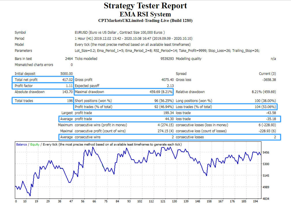
The first stage of analysis is to look at the key areas of the Strategy Tester report.
In terms of analyzing your EA and strategy, the following sections of the report are the most important:
Total Net Profit
The result of all trades, this represents the difference between “Gross profit” and “Gross loss”.
This shows whether a system will be worthwhile or not.
Profit Factor
This is the ratio between the gross profit and the gross loss. A value of 1 is breakeven, a negative number means the system lost overall and a number greater than 1 means the system is profitable. The higher the number, the better, although a very high profit factor could show a system has been curve fitted.
Maximal Drawdown
The total percentage of account equity lost during the worst drawdown period. This is useful because it gives you an idea of what a bad drawdown looks like, and allows you to consider whether you could deal with such a situation psychologically.
Total Trades
The total amount of trades placed, this shows you if there is enough data in your test for statistical significance.
Profit Trades (% of Total) & Loss Trades (% of Total)
The percentage of profitable and unprofitable trades. Again, this is useful in determining if you can handle trading the system. For example if the win rate is less than 30%, would you be able to deal with it mentally?
Average Profit Trade & Average Loss Trade
The average profit and loss value of all trades trade. This allows you to quickly see your risk:reward – ideally the profit value will be higher than the loss value.
Average Consecutive Wins & Average Consecutive Losses
The average amount of profitable or unprofitable consecutive trades. Again, if there are typically many losing trades in a row, will you be able to psychologically handle trading this system with real money?
Advanced Analysis
Having analyzed a report, if it meets our requirements then we can apply further, advanced analysis to look for further clues as to how the system might perform going forward.
To conduct the tests that follow, we will use the free version of StrategyQuant’s QuantAnalyzer program.
Analyzing By Day, Hour & Month
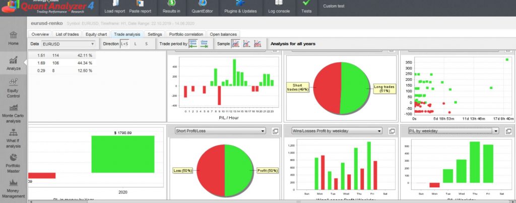
An excellent set of features in the QuantAnalyzer are the “Analyze” tools.
This provides an array of analysis tools, but some of the most helpful are found under the “Trade analysis” tab:
Using this, we can drill down and find useful information about our strategy. As we mentioned in an earlier lesson, we can now look for specific times of day, days of the week or months when we might not want to trade our system. These can be programmed as variables into our EA.
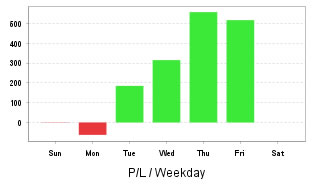
For example, it appears our example system does not make any money on Sundays or Mondays:
Therefore it may be advisable to not trade on these days at all.
It is definitely worth spending some time with the “Analyze” tools to give you greater insight into your system.
Monte Carlo Analysis
Monte Carlo simulation is an advanced risk analysis tool. It allows you to get a more accurate picture of the performance of a trading strategy than a standard backtest report can provide.
A Strategy Tester report shows the results of a series of trades, in a specific order, but we don’t know what might happen to the strategy’s performance going forward. If, for example, a lot more losing trades occurred consecutively than were shown in the backtest, what type of drawdown will that incur? What is the probability that you could experience a drawdown that is larger than you expect, or a streak of losing trades longer than you expect?
Monte Carlo analysis allows you to scramble the order of the trades in a backtest to provide a better understanding of possible future performance, based on the assumption that future trades will have similar characteristics to historical trades, but in an unknown order.
The results allow you to determine the probabilities of profits and drawdowns. You can also analyze the probability of your trading account being wiped out completely.
Monte Carlo Analysis in QuantAnalyzer
In order to understand how QuantAnalyzer works, please watch the video at the top of this page if you haven’t already done so.
After running a Monte Carlo simulation on one of our strategies, the resulting equity graph is generated:
This shows all possible possibilities for performance of the system with the backtested trades in random order, and with a 1% probability of a trade being skipped.
The lowest line on the graph represents the worst possible performance of the system, whereas the upper line represents the best possible performance.
Risk of Ruin
This allows us to view the probability of the system wiping out the trading account based on the initial trade capital size and money management rules.
This is useful for determining whether a system may be unsuitable for trading, if there isn’t enough initial capital available to do so:
Predict
This section allows you to predict how the strategy might perform in the future.
The pink section on the chart shows the possible range in which the equity could increase or decrease, depending on the existing Monte Carlo simulation. Again, the bottom area shows the worst case scenario, whereas the upper area shows the best case scenario.
Verify
This mode can be used to verify if the real performance of the strategy falls inside the predicted range computed using Monte Carlo simulation. In the example below, we can see that the backtest is within the range projected by the Monte Carlo simulation:
Conclusion
As you can see, analysis of your backtests is extremely important. Advanced analysis can give us more confidence in a trading system, and can reveal information based on statistical probability that we otherwise wouldn’t know.
It is, however, important to note that you need to test on tick data, otherwise the advanced analysis will be based on unreliable backtests, and the advanced information generated from these Strategy Reports will also be unreliable.


